What is Quantum Computing?

1. Abstract

This article is my attempt to explain and understand what is quantum computing. As I am new to the subject and learning it myself, the information contained in the article could be potentially wrong. But it would be an interesting exercise to write this brief article documenting what I think it is – based on just a few hours of reading a book – and see if my understanding was correct as time passes by and I learn more about the subject.

2. So what is it?

I’d like to give the analogy of Fourier Optics as for me analogies are the best way I understand things. From Wikipedia, see the section titled Fourier transforming property of lenses: If a transmissive object is placed one focal length in front of a lens, then its Fourier transform will be formed one focal length behind the lens. So if you want to compute a 2D Fourier Transform (FT) you could do it the conventional way where you write some code in your favorite programming language, run it on a computer and get the result. Or another way to “compute” the FT would be to use a lens and its Fourier transforming property. The Wikipedia article goes on: “All FT components are computed simultaneously – in parallel – at the speed of light. As an example, light travels at a speed of roughly 1 ft (0.30 m) / ns, so if a lens has a 1 ft (0.30 m) focal length, an entire 2D FT can be computed in about 2 ns (2 x 10⁻⁹ seconds). If the focal length is 1 in., then the time is under 200 ps. No electronic computer can compete with these kinds of numbers or perhaps ever hope to, although supercomputers may actually prove faster than optics, as improbable as that may seem. However, their speed is obtained by combining numerous computers which, individually, are still slower than optics.”

Quantum Computing is completely analogous. The behavior/evolution of quantum particles or a quantum system can be described by operation of matrices – linear algebra. The equations governing quantum mechanics are linear – that is why a quantum particle or system can exist in superposition of states because for a linear equation if X and Y are solutions, then any linear combination of X and Y is also a solution. So say you have a problem which requires you to calculate something which is nothing but basically a sequence of special matrix operations. You could do it the conventional way, or if you could build a quantum system (circuit), you could let it evolve and monitor (measure) it to get the answer – that is basically a quantum computer.

Conventional computers are Turing machines which evaluate Boolean logic. Quantum computers evaluate matrix operations and using the property of entanglement they can run many inputs in parallel. Boolean logic is composed of a handful of operators – OR, AND, NOT and combinations of those. In case of QC we have special matrices that form the building blocks. Conventional computers speak the language of Boolean Logic. Quantum Computers speak and understand the language of matrix computations.

There are two things from which quantum computers derive all their power – superposition and entanglement.

3. Challenges

The challenge with QC is that building a quantum system is hard and the difficulty increases as the number of particles (i.e., number of qubits) to be entangled increases. The system can quickly get disentangled due to decoherence so the challenge is in being able to build and control the system. This is the hardware challenge. Another challenge is finding useful problems that can be expressed as quantum computations. Computing 2D FT is is very useful problem in image processing. We need to find useful problems that can be expressed as quantum (err.. matrix) computations. This is the software challenge.

A bibliography of quantum algorithms is available at https://quantumalgorithmzoo.org/ – these are essentially the use-cases. If you have a problem that can be reduced or mapped to one of these cases, then you can use a QC to solve it. However there is a catch here that many algorithms require using a number of qubits which is out of reach of today’s quantum computers. E.g., Shor’s algorithm for factorization is a famous example of quantum computation that can be used to break RSA cryptography. But it requires a # of qubits which is out of reach of today’s QC. The hardware challenge is being solved by companies like Google and IBM. They will make quantum computers and make them accessible via the cloud just like we can access GPU and other beefy machines today using AWS or other cloud providers.

One of the things I have noticed in my limited exploration of this topic is that the current software libraries for quantum computation (Google’s Cirq and Microsoft’s Q# are some examples) are high-level languages but the code is written to express a “low-level” quantum circuit. Its like asking you to program a classical computer by writing code to create the underlying Boolean Logic circuit – no one does that these days. I wonder if in future the libraries will evolve so that one does not have to write a “low-level” circuit. Maybe its the way it is because quantum computer has an advantage over classical computer only when the computation can be expressed as a quantum circuit – basically a sequence or flowchart of special matrix operations – special because not every matrix operation is qualified to be permitted in a quantum circuit. Only special matrix operations are permitted – in particular the matrices must be invertible.

4. What does Google’s recent Quantum Supremacy claim mean?

Google’s recent announcement of Quantum Supremacy made big news every where. What is it about? It basically demonstrated that they were able to build a 54-qubit processor and put it to some use. Its about the hardware challenge. Building a QC becomes very difficult as the number of qubits increase because its very difficult to keep them entangled and pure and prevent them from getting disentangled as the computation progresses (the depth of the circuit). The problem they solved was not interesting per se – they sampled the probability distribution resulting from a random circuit. The input to the problem is a state vector that can take on 2n possible values where n is the number of qubits. This state vector essentially undergoes transformation by a random quantum circuit to yield the output vector. This output vector can be in so many states and we are interested in finding or rather sampling from its probability distribution. Google team did this computation using both a quantum computer as well as a classical computer. They then compared result of QC with result of classical computer to validate and verify that the QC was giving correct results – this would not have happened if the qubits had gotten disentangled. Sotheir achievement was in being able to demonstrate a system that could control and keep 54 qubits in entanglement through the course (depth) of their circuit. Ultimately as n increases they reach a point where classical calculation becomes infeasible.

5. Quantum Computing: Pop Quiz

Think you understand quantum computing. See if you can answer following question:

In QC, it is said that the quantum state of N qubits can be expressed as a vector in a space of dimension 2N. E.g., if you have 1 qubit there are two state vectors (0,1) and (1,0) which are written as |0> and |1> respectively. For a system of 2 qubits, there are 4 state vectors (0,0,0,1), (0,0,1,0), (0,1,0,0) and (1,0,0,0) written as |00>, |01>, |10>, |11>. Note that in each case, all entries are zero except 1. 2N seems like a big space but given a vector in this space – all components will be zero except 1. So there are only 2N possible values the state vector can take. So why don’t we say the space is N dimensional? A N-bit string has 2N possible values. To make the question more provocative, the total memory required to store the state vector is claimed to be of the order of 2N. This quickly becomes out of reach when we try to do classical simulation and is at the heart of Google’s Quantum Supremacy. For system of only 50 qubits we would need petabytes of storage to store the state vector. But we only need N bits to store the position of the 1 in the state vector – rest all entries are zero. So what gives?

Posted in Science | Leave a comment

Generating random passwords

[software]


here is a useful command to generate a random password from the command line

$ openssl rand -base64 8
BTz1bGHrs6s=

change the last argument to change the length of the password

Posted in Software | Leave a comment

How to change the maximum file size you can upload to wordpress

Spent a lot of time figuring this out and trying out different things suggested by different sites so thought would make a note of it. Its actually quite simple once you know what you need to do. All you need to do is to change the values of two variables `upload_max_filesize` and `post_max_size` in two places `/etc/php/7.2/apache2/php.ini` and `/etc/php/7.2/cli/php.ini`

$ sudo vi /etc/php/7.2/apache2/php.ini
$ sudo vi /etc/php/7.2/cli/php.ini

we also need to restart the server

$ sudo systemctl restart apache2

Files are uploaded to directory given by [wp_upload_dir](https://developer.wordpress.org/reference/functions/wp_upload_dir/)

To see media files https://wordpress.stackexchange.com/a/95683/29199

“`
Select * from wp_posts where post_type = ‘attachment’;
“`

Troubleshooting: wordpress uses following code to determine the max file size shown in the UI

“`
wp-admin/includes/media.php: $max_upload_size = wp_max_upload_size();
“`

https://developer.wordpress.org/reference/functions/wp_max_upload_size/

in

“`
function wp_max_upload_size() {
$u_bytes = wp_convert_hr_to_bytes( ini_get( ‘upload_max_filesize’ ) );
$p_bytes = wp_convert_hr_to_bytes( ini_get( ‘post_max_size’ ) );

/**
* Filters the maximum upload size allowed in php.ini.
*
* @since 2.5.0
*
* @param int $size Max upload size limit in bytes.
* @param int $u_bytes Maximum upload filesize in bytes.
* @param int $p_bytes Maximum size of POST data in bytes.
*/
return apply_filters( ‘upload_size_limit’, min( $u_bytes, $p_bytes ), $u_bytes, $p_bytes );
}
“`

One tip is that above just controls the value shown in the UI. E.g., you can override the function so that it returns 1G but if the settings in .ini files are not changed, the server (apache) will not let you upload files larger than what the .ini file says.

Posted in Software | Tagged | Leave a comment

San Diego – 5 day itinerary

Maritime Museum

Where To Stay: Hotel Republic. It is in the Financial District (downtown), walking distance to the Marina, Amtrak, Aaharn and Karl Strauss Brewing Company.

Where to buy tickets: Go City pass or Costco.

Transportation: Recommend to take Uber and not rent a car since there is $50 valet parking charge at hotel per day.

Day 1: Arrive at hotel. Buy groceries from Ralph’s nearby and head to Coronado island in the evening (Hotel Del Coronado). Coronado is the happening place in San Diego. More happening than Downtown San Diego itself. And Hotel Del Coronado is a place to visit. Eat at Miguel’s Cocina near Hotel Del Coronado.

Day 2: San Diego Zoo. Or do the Safari Park instead if you have already been to some zoo couple of times. The Zoo comes up as the top attraction of San Diego. Its not bad but comparable to Woodland Park Zoo (Seattle) so can be easily substituted for something else like the Safari. They have lot of monkeys but oddly there were no gorillas. The best exhibit I found was that of Asian Leopards. They have at least 4 of them and they were very active. You do feel a sense of guilt watching the animals in captivity (esp. the birds which are meant to soar in the skies). Dinner at Aaharn. Aaharn is the best place for budget conscious. The food is good and it cost only $20 for 2 people. Rest of the places were 3x expensive. If you are staying at Hotel Republic you could eat at Aaharn throughout your trip.

Day 3: La Jolla Cove. Start at the children’s pool and walk to La Jolla Cove and the Cave Store. Check out the cave and then head over to Salk Institute. Have lunch at Salk Cafeteria (good food and very cheap) and then go to the Gliderport. Do paragliding there. It is costly ($175 + $100 for photos and video) but worth it if you have never done it before. Also the best views of the ocean are from here. Then explore UCSD campus nearby. Dinner at Karl Strauss.

Salk Institute

Day 4: Sea World. There are 2 main roller coaster rides – Electric Eel and Manta. Both are lot of fun. Then there is Tidal Twister, Journey to Atlantis and Shipwreck Alley which are fun as well. If you have been to another Sea World then might want to substitute with Legoland. Stroll around the marina in the evening.

Day 5: Check out from hotel. USS Midway. Amazing experience. They have dozens of fighter and bomber planes plus you can take a tour of the ship all the way from the bridge to the engine room. You can see the dining hall, admiral’s desk, kitchen, laundry, radio room, conference rooms, mess, supply room, pretty much everything. They have interesting talks where they explain crew in yellow jackets direct the planes, the crew in red jacket checks ammunition, white jacket checks safety and so on. They have a place where you can park your luggage in case you are taking flight back home in the afternoon.

Gaslamp Quarter is supposed to be an attraction but I found it passable.

Map: https://goo.gl/maps/RFpW8khiZZUmXrRx9

Posted in Travel | Leave a comment

Decoding the algorithm behind Levels.fyi

I have been quite impressed with Levels.fyi website which shows a mapping of career levels between companies. E.g., what does a level 66 in Microsoft map to in Uber? How does it do it? How would I do it? Let’s say we have data from users when they switch jobs that tells us the level of the person in company A and what level the person joined in company B. So this would e.g., give us a table of the form:

So to get a mapping between Microsoft and Uber, for each level x in Microsoft:

  • filter data and select rows where From = Microsoft, From_Level = x, To = Uber
  • and average the To_Level column of rows from previous step

That gives mapping of level x in Microsoft to Uber. Call it M(Msft,x,Uber) = M(from,level,to)

This will not work. To see why, consider the fact that when people switch they usually accept a lateral level or better yet level up. Rarely do they level down. So when we run the above algorithm, we might get a table that looks like (assuming people aggresively level up when they switch):

and if we re-run the algorithm, but switch the roles of Microsoft and Uber i.e., we compute M(Uber,x,Msft) we might get a mapping that looks like:

Clearly this is wrong. It implies level 63 at Microsoft = level 66 at Microsoft. For a correct mapping, we require

M(Uber, M(Msft,x,Uber), Msft) = x

How to find such a M? Well, the solution is simple. Plot all the points where people have switched between Microsoft and Uber on a 2D graph and fit a straight line through them. One might be tempted to do fancy things like clustering to handle non-linearity but it will only make things worse. Hint: Try making a scatter plot where candidates constantly level up. How will you cluster?

Levels.fyi goes beyond this: it actually allows one to select more than two companies and instantly see the mapping between levels. How could this be possible? Well, the answer is simple. In practice it does none of the above. In reality, all levels are mapped to compensation and using compensation as a common hidden variable, it is very easy to get a mapping of levels between arbitrarily selected companies. So in the end, level is nothing but a proxy for money. There you have it. In fact, the table From, From_Level, To, To_Level doesn’t even exist. When levels.fyi collects data, their form only records compensation and level at current company, not the levels when a person switches from company A to B.

Further Reading

Posted in Career, Money | Leave a comment

Roth vs Traditional 401k – final take

This is my final take on Roth vs. Traditional 401k in which I extend the previous model to include two new variables:

  • a different tax rate t_2 for money withdrawn from 401k (the expectation is that you will be in a lower tax bracket during retirement) and
  • a variable e to denote the expenses in a year. These expenses need to be deducted from the amount that is invested in the ordinary non-tax sheltered account.

with these two variables, the new calculations for Roth vs. traditional are as follows:

Roth 401k

Total = Roth = (1+r)^N c + (p - c - e - f(p))(1 + r')^N

where:
f(x) is a function that computes tax on x, and
r' = r(1 - t_1) is the reduced rate of return that money in non-tax sheltered account earns
t_1 will be the marginal tax rate (bracket)

Traditional 401k

Total = Trad = (1+r)^N c (1 - t_2) + (p - c - e - f(p-c))(1 + r')^N

where:
t_2 = expected tax rate at time of withdrawal in retirement

Let’s see what we get if we subtract the two:

D = Roth - Trad = (1+r)^N c t_2 - (f(p) - f(p-c))(1 + r')^N
Now recall f is simply the function which computes tax, so f(p) - f(p-c) = t_1 c giving
D = (1+r)^N c t_2 - (1 + r')^N t_1 c
simplifying:
D = ((1+r)^N t_2 - (1 + r')^N t_1) c
For D > 0 
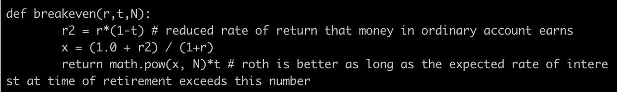
(i.e., better to invest in Roth), we get a simple formula
(1+r)^N t_2 > (1 + r')^N t_1
This looks like a linear relationship in t_1 and t_2 but isn’t since r' is a function of t_1. The variables p,c,e have cancelled out and we see that the factors that influence whether you should choose Roth vs. Traditional 401k are:

  • your current tax bracket t_1
  • your expected tax bracket during retirement t_2
  • expected rate of return on investment r
  • time to retirement N

We can write a small function that gives us the breakeven point when both Roth and Traditional will give same return:

Let’s see what it gives:

Plot of breakeven point vs. N (# of years till retirement) with r=0.08 
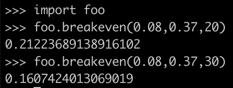
and two different values of t_1

Enough math. Can I get it in English please? Investing in Roth makes sense if you are young (i.e., N ↑) or in a low tax bracket (t_1 ↓). For most people, both these events happen at the same time. To use the graph above, calculate the # of years you have till retirement (x-axis) and your expected tax bracket in retirement (y-axis). That should give you a point on the graph. If that point is above the curve, you are better off investing in a Roth 401k.

Conclusion: Go Roth when you are young and switch to Traditional 401k once you cross 40-45 years of age. For most people that represents mid-point of their career. Thus, in other words, the conclusion is to split evenly between Roth and Traditional 401k. Choose Roth for first-half of your career and Traditional for the second half.

of course, again all this is just bookish exercise for fun. Code is here.

Posted in Money | Leave a comment

Roth vs Traditional 401k – take two

There is a subtle bug in my original post on Roth vs. Traditional 401k. The bug being that in Roth 401k, we pay taxes upfront but we still get to invest full contribution amount that grows tax-free. The bug is so subtle that let’s do another analysis that will make it clear. Let

p 
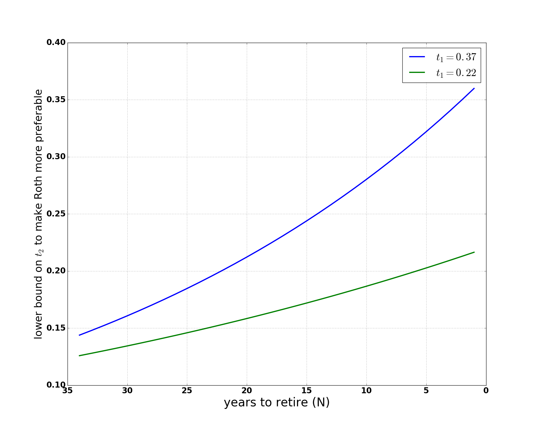
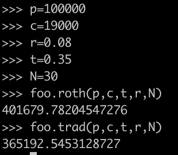
= principal amount = salary earned in a year = $100,000 as example
c = contribution amount to 401k = $19,000 for 2019 whether it be roth or traditional
r = rate of return on investment = 0.08 as example
t = tax rate = 0.35 as example
N = # of years money is invested

Roth 401k
We start with p. c goes into 401k account. That leaves us with p-c in ordinary account. Next we pay tax on the full p which further reduces it to (1-t)p-c. Call this A. This amount can be invested just like we invest the money in a 401k. The only difference is that in ordinary account we will have to pay tax on earnings every year. I leave it as an exercise for reader to prove that the annual tax incurred in the ordinary account basically has the effect of reducing r by a factor of 1-t so that at end of N years, A invested in ordinary non-tax sheltered account will grow as (1+r(1-t))^N A
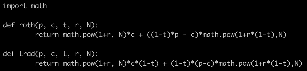
. The money in 401k grows as (1+r)^N c and can be withdrawn tax free. So at the end we have

Total = (1+r)^N c + (1+r(1-t))^N ((1-t)p-c)

Traditional 401k
We start with p. c goes into 401k account. That leaves us with p-c in ordinary account. Next we pay tax on only p-c which reduces it to (1-t)(p-c). This becomes the new A. This amount can be invested just like we did earlier. In case of traditional 401k, the money in 401k will grow to (1+r)^N c but we will have to pay tax on this at time of withdrawal. So at the end we have

Total = (1+r)^N c (1-t) + (1+r(1-t))^N (1-t)(p-c)

The total amount we end up with is not the same in the two cases. I wrote a small script to compute the two totals

when I run this script:

so Roth seems to be better. But beware, this is just bookish exercise that assumes t to be same in case of retirement vs. not. In reality what is expected is that in retirement your tax rate should be lower than the tax rate when you are earning. In that case traditional 401k might turn out to be better.

Posted in Money | Leave a comment

Traditional vs Roth 401k

Let p be amount invested over N years. r = rate of return. t = tax rate.

Roth 401k
You pay taxes upfront. That reduces p to (1-t)p. After N years this becomes (1+r)^N(1-t)p which you can withdraw tax free.

Traditional 401k
You don’t pay any taxes on p. After N years the amount becomes (1+r)^Np. Now when you withdraw it, you pay tax and so the net amount becomes (1+r)^Np(1-t) which is same as earlier.

Of course, the catch is the assumption that t remains same in both cases.

Posted in Money | Leave a comment

Understanding Docker Volumes

Docker volumes are a complicated beast. They can be created using the `docker volume create` command or in the docker-compose.yaml file under the volumes section. E.g.:

What this does is create persistent storage on the host that 1. does not get deleted when a docker container stops and exits and 2. that can be used to share data amongst containers.

To see a list of volumes on your machine, run:
“`
$ docker volume ls
“`

To get details of a volume, run (to give an example):

The volumes are not created as regular directories on the filesystem that can be accessed using familiar unix commands. E.g., if you try to list the mountpoint in above:

In fact there is no `/var/lib/docker`. To “get” to the volume requires some steps taken from https://forums.docker.com/t/host-path-of-volume/12277/6:

  1. First (on the mac) run `$ screen ~/Library/Containers/com.docker.docker/Data/vms/0/tty`. This should open an absolutely blank screen. `~/Library/Containers/com.docker.docker/Data/vms/0/tty` itself is a link to `/dev/ttys000`
    “`
    $ ls -al ~/Library/Containers/com.docker.docker/Data/vms/0/tty
    lrwxr-xr-x 1 sjain68 staff 12 Nov 5 09:03 /Users/sjain68/Library/Containers/com.docker.docker/Data/vms/0/tty -> /dev/ttys000
    “`
  2. Now ls the mountpoint you found earlier
  3. To exit the screen type `Ctrl+A` followed by `:quit`. DO NOT type `exit` as it will mess you up. https://stackoverflow.com/a/2308595/147530

    Screen Shot 2019-11-05 at 11.25.37 AM
    the `tty` is not a file. It is a device.
    “`
    $ ls -al /dev/ttys000
    crw–w—- 1 sjain68 tty 16, 0 Nov 5 11:13 /dev/ttys000
    “`

Posted in Software | Leave a comment

Cryptogen 1.4.3 Bugs

As is common for Fabric, the cryptogen utility (1.4.3) has various bugs as of this writing:

  1. The most important bug is that the admincerts folder is empty. see https://jira.hyperledger.org/browse/FAB-16933
  2. The next bug (FAB-16936) is that if you are enabling Node OUs, the OU for the orderer’s admin has OU=client instead of OU=admin. Example:
    Subject: C=US, ST=California, L=San Francisco, OU=client, CN=Admin@foo.com
    For comparison, The peers admin have OU=admin set correctly:
    Subject: C=US, ST=California, L=San Francisco, OU=admin, CN=Admin@bar.com
Posted in Software | Tagged | Leave a comment