3. Add string (e.g., *) to end of every line (ref):
:%norm A*
4. Add string to beginning of every line:
:%norm I*
5. delete last character on every line:
:%s/.$//
6. Find your vi config file by typing:
vim --version
On Mac OS I see:
system vimrc file: "$VIM/vimrc"
     user vimrc file: "$HOME/.vimrc"
 2nd user vimrc file: "~/.vim/vimrc"
      user exrc file: "$HOME/.exrc"
       defaults file: "$VIMRUNTIME/defaults.vim"
  fall-back for $VIM: "/usr/share/vim"
You can now edit $HOME/.vimrc to create global configuration. e.g., to set tab spaces to 4 (instead of 8):
This post describes results of a test to compare the performance of MySQL vs. Postgres on the TPC-C Benchmark for OLTP workloads. The tool used for performance benchmarking was sysbench-tpcc. Note that sysbench-tpcc simulates a TPC-C like workload not exactly TPC-C. The results cannot be compared to official benchmark. sysbench-tpcc is not validated and certified by the TPC organization.
That said, for the impatient the performance was the same across MySQL and Postgres with very little difference. Both gave a TPS of 50 tx/s on a machine with 8 vCPU and 32 GB RAM. I felt this was quite remarkable. Details follow.
The command took 45 min to run. It generates about 1000 tables. To calculate the total size first we have to compute statistics:
mysql> use sysbench;
SET @tables = NULL;
SELECT GROUP_CONCAT(table_name) INTO @tables
FROM information_schema.tables
WHERE table_schema = 'sysbench';
SET @tables = CONCAT('ANALYZE TABLE ', @tables);
PREPARE stmt FROM @tables;
EXECUTE stmt;
DEALLOCATE PREPARE stmt;
Then we can get cumulative data size:
mysql> SELECT SUM(data_length + index_length) / 1024 / 1024 AS 'DB Size (MB)' FROM information_schema.tables WHERE table_schema = 'sysbench';
+-----------------+
| DB Size (MB)    |
+-----------------+
| 325088.09375000 |
+-----------------+
1 row in set (0.04 sec) --> This is 3x more than postgres as we see later

mysql> SELECT SUM(data_length) / 1024 / 1024 AS 'DB Size (MB)' FROM information_schema.tables WHERE table_schema = 'sysbench';

+-----------------+
| DB Size (MB)    |
+-----------------+
| 294732.06250000 |
+-----------------+
1 row in set (0.04 sec)

mysql> SELECT SUM(index_length) / 1024 / 1024 AS 'DB Size (MB)' FROM information_schema.tables WHERE table_schema = 'sysbench'
;
+----------------+
| DB Size (MB)   |
+----------------+
| 30356.03125000 |
+----------------+
1 row in set (0.05 sec)
We keep all the default settings provided by GCP and run the workload using:
Before running the benchmark we did two things: VACUUM ANALYZE the database:
VACUUM ANALYZE;
VACUUM reclaims storage occupied by dead tuples. In normal PostgreSQL operation, tuples that are deleted or obsoleted by an update are not physically removed from their table; they remain present until a VACUUM is done. Therefore it’s necessary to do VACUUM periodically, especially on frequently-updated tables. In this case since we just created the database it was not necessary.
The second thing we did was to tweak the default settings to following:
This was done based on what I read here. I think the main thing to note is enabling the wal_compression. Not sure how much of a difference the other settings make. Anyway the test was then run as follows:
SQL statistics:
    queries performed:
        read:                            2310777
        write:                           2398055
        other:                           356420
        total:                           5065252
    transactions:                        178154 (49.45 per sec.)
    queries:                             5065252 (1405.93 per sec.)
    ignored errors:                      785    (0.22 per sec.)
    reconnects:                          0      (0.00 per sec.)

General statistics:
    total time:                          3602.7877s
    total number of events:              178154

Latency (ms):
         min:                                  155.87
         avg:                                 1131.91
         max:                                 5513.34
         95th percentile:                     2632.28
         sum:                            201655147.95

Threads fairness:
    events (avg/stddev):           3181.3214/45.27
    execution time (avg/stddev):   3600.9848/0.71
So here we are: basically the same TPS! In fact the results are so similar (even the latency is the same) that I had to check I did not mistakenly run both tests on the same database. Which one do you like? The elephant or the dolphin? Let me know in your comments.
Serializable Level
Below are results of MySQL vs Postgres when running with 20 concurrent threads and when transaction isolation level is set to SERIALIZABLE. We use exact same config as before except that --threads=20 and --trx_level=SER
MySQL:
SQL statistics:
    queries performed:
        read:                            827056
        write:                           858380
        other:                           127206
        total:                           1812642
    transactions:                        63573  (17.65 per sec.)
    queries:                             1812642 (503.14 per sec.)
    ignored errors:                      290    (0.08 per sec.)
    reconnects:                          0      (0.00 per sec.)

General statistics:
    total time:                          3602.6817s
    total number of events:              63573

Latency (ms):
         min:                                  156.71
         avg:                                 1132.83
         max:                                 4715.93
         95th percentile:                     2632.28
         sum:                             72017367.32

Threads fairness:
    events (avg/stddev):           3178.6500/42.11
    execution time (avg/stddev):   3600.8684/0.73
Postgres:
SQL statistics:
    queries performed:
        read:                            822696
        write:                           854108
        other:                           127148
        total:                           1803952
    transactions:                        63390  (17.60 per sec.)
    queries:                             1803952 (500.85 per sec.)
    ignored errors:                      445    (0.12 per sec.)
    reconnects:                          0      (0.00 per sec.)

General statistics:
    total time:                          3601.7746s
    total number of events:              63390

Latency (ms):
         min:                                  156.15
         avg:                                 1136.06
         max:                                 5005.31
         95th percentile:                     2680.11
         sum:                             72014634.91

Threads fairness:
    events (avg/stddev):           3169.5000/35.23
    execution time (avg/stddev):   3600.7317/0.59
Again results are practically the same! No difference at all. (The most visible difference is in the errors which is 290 for MySQL vs 445 for Postgres). I had to double-check I did not execute the tests against the same server. And believe me, I did not. I find this quite remarkable because the internals of MySQL and Postgres are subtly different when it comes to storage and managing concurrency. First, MySQL uses a clustered index for its storage whereas Postgres uses a heap. Second, when it comes to managing concurrency at SERIALIZABLE level, MySQL uses a combination of MVCC and 2PL (2 phase locking) whereas Postgres uses Serializable Snapshot Isolation (SSI). And third, MySQL is using a thread per connection whereas Postgres spawns a new process per connection. In terms of memory usage I found Postgres was taking up 21.3 GiB whereas MySQL was taking a little more 26.89 GiB.
Below is a snapshot of sample queries being executed against the database as we run sysbench-tpcc.
DELETE FROM new_orders8 +
WHERE no_o_id = 2114 +
AND no_d_id = 1 +
AND no_w_id = 18
COMMIT
SELECT s_quantity, s_data, s_dist_05 s_dist +
FROM stock10 +
WHERE s_i_id = 80424 AND s_w_id= 77 FOR UPDATE
SELECT s_quantity, s_data, s_dist_10 s_dist +
FROM stock7 +
WHERE s_i_id = 1469 AND s_w_id= 1 FOR UPDATE
SELECT s_quantity, s_data, s_dist_05 s_dist +
FROM stock5 +
WHERE s_i_id = 1875 AND s_w_id= 13 FOR UPDATE
INSERT INTO new_orders6 (no_o_id, no_d_id, no_w_id) +
VALUES (3012,5,58)
UPDATE stock1 +
SET s_quantity = 53 +
WHERE s_i_id = 10556 +
AND s_w_id= 41
SELECT o_c_id +
FROM orders6 +
WHERE o_id = 2115 +
AND o_d_id = 10 +
AND o_w_id = 6
SELECT s_quantity, s_data, s_dist_03 s_dist +
FROM stock6 +
WHERE s_i_id = 50357 AND s_w_id= 17 FOR UPDATE
SELECT no_o_id +
FROM new_orders9 +
WHERE no_d_id = 7 +
AND no_w_id = 31 +
ORDER BY no_o_id ASC LIMIT 1 FOR UPDATE
SELECT i_price, i_name, i_data +
FROM item5 +
WHERE i_id = 48208
INSERT INTO order_line5 +
(ol_o_id, ol_d_id, ol_w_id, ol_number, ol_i_id, ol_supply_w_id, ol_quantity, ol_amount, ol_dist_info)+
VALUES (3011,6,37,13,42417,37,3,55,'dddddddddddddddddddddddd')
SELECT c_first, c_middle, c_last, c_street_1, +
c_street_2, c_city, c_state, c_zip, c_phone, +
c_credit, c_credit_lim, c_discount, c_balance, c_ytd_payment, c_since +
FROM customer7 +
WHERE c_w_id = 92 +
AND c_d_id= 7 +
AND c_id=764 FOR UPDATE
BEGIN
SELECT i_price, i_name, i_data +
FROM item10 +
WHERE i_id = 69582
SELECT i_price, i_name, i_data +
FROM item9 +
WHERE i_id = 71983
INSERT INTO history10 +
(h_c_d_id, h_c_w_id, h_c_id, h_d_id, h_w_id, h_date, h_amount, h_data) +
VALUES (6,67,1559,6,67,NOW(),3072,'name-mzlqb name-cvffw ')
INSERT INTO order_line9 +
(ol_o_id, ol_d_id, ol_w_id, ol_number, ol_i_id, ol_supply_w_id, ol_quantity, ol_amount, ol_dist_info)+
VALUES (3014,2,59,12,84480,59,10,372,'rrrrrrrrrrrrrrrrrrrrrrrr')
UPDATE warehouse2 +
SET w_ytd = w_ytd + 998 +
WHERE w_id = 73
SELECT i_price, i_name, i_data +
FROM item8 +
WHERE i_id = 33257
(21 rows)
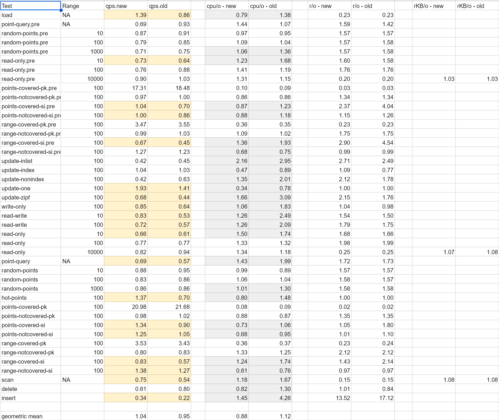
Also of interest
below spreadsheet is from this article. The qps.new column tracks performance ratio of PG vs MySQL. Results are similar. Overall the geometric mean is 1.04 reflecting no significant difference between the two.
On closer inspection of above spreadsheet, we see most of the time its MySQL that is better. There are a few outliers where PG performs vastly better like points-covered-pk where the ratio is 20. What do we get if we instead take the median of the results?
– more popular and widely used – more learning resources – uses threads instead of processes for connections – better indexing. secondary indexes point to primary index. – read Uber’s blog why they switched from Postgres to MySQL. – Postgres has no show create table command that comes with MySQL – Postgres has no unsigned int
– materialized views (although they don’t auto-refresh) – multiple index types (B-Tree, Hash, BRIN, GIN, GIST) – custom types – arrays – extensions (plugins) – stored procedures can be written in multiple languages – generally accepted to have more bells and whistles than MySQL – developer community seems to be more friendly. – most loved and wanted database on SO – do what you want with it license. no strings attached.
Performance-wise I think both are close. There are popular tools like sysbench to compare performance but I feel the test cases are a bit contrived and don’t reflect real-world usage. Also the winner might change from year to year like the car rankings in consumer reports.
There is lots of good stuff in above article. Even though the underlying architecture between MySQL vs Postgres is very different, yet they give similar levels of performance. This is because as Nasser says in his article, no solution is without its problems. What we gain in one area is sacrificed by what we lose in another. However, MySQL’s design of using threads is undoubtedly better than Postgres’s design of using processes. You can have many more threads running on a system than processes. And inter-process communication is much more costly than communication between threads (refer this for some more details). I even like the idea of using a clustered index (MySQL) vs. heap (Postgres) to store the data. It leads to less write-amplification as Uber noted in their blog. And when it comes to concurrency, I believe that under very high contention 2PL (MySQL) would perform better than SSI (Postgres) as it would lead to less CPU wastage. Greg Kemnitz, Staff Database Engineer at Google writes: “The one huge advantage of MySQL over Postgres is in the InnoDB (and XtraDB) storage engine, which is extremely good for 24/7 OLTP environments of the sort you’d have in a large production website or customer-facing application. Postgres’ need for a storage garbage collector (VACUUM) basically kills it for these types of applications, which is the biggest reason why Uber switched from Postgres to MySQL“. Its interesting that from a theoretical perspective, MySQL seems to be the better database. Yet when it comes to practice, more people love Postgres than MySQL. Try doing a web search on terms like “I love MySQL” or “MySQL sucks” or “I love Postgres”, “Postgres sucks”, “Why MySQL is better than Postgres”, “Why Postgres is better than MySQL” etc. Getting answers to questions (think of this as customer support) is also easier with Postgres with their user-friendly mailing list instead of a clumsy web-only forum with MySQL that requires Oracle login. And the best part about Postgres is that you can do whatever you want with it. You don’t have to ask for any permission or obtain a license. That is why it is becoming more popular and companies like Microsoft (with Citus acquisition) are now actively contributing in a big way to the project.
What do you think? Which one do you prefer? The elephant or the dolphin? Let me know.
Addendum: Comparing MySQL and Postgres indexes to Chapters 10 and 9 of File Structures by Michael Folk et. al.
Recently I came across this excellent book. AFAIU, Postgres index corresponds to the index covered in Chapter 9 of this book (referred to as a B tree by the authors) whereas MySQL index corresponds to Chapter 10 (referred to as B+ tree by the authors). The authors write (Ch 9, p. 401):
In this book, we use the term B+ tree to refer to a somewhat more complex situation in which the data file is not entry sequenced (an entry sequenced file = Postgres’ heap in which elements appear in order in which they are inserted into the database) but is organized into a linked list of sorted blocks of records (this is exactly like MySQL’s clustered indexAFAIU).
The great advantage of the B+ tree organization is that both indexed access and sequential access are optimized.
B trees provided excellent access performance, but there was a cost: no longer could a file be accessed sequentially with efficiency. Fortunately, this problem was solved almost immediately by adding a linked list structure at the bottom level of the tree.
Now I understand what Nasser is referring to when he writes:
I think MySQL is the winner here for range queries on primary key index, with a single lookup we find the first key and we walk the B+Tree linked leaf pages to find the nearby keys as we walk we find the full rows.
Postgres struggles here I think, sure the secondary index lookup will do the same B+Tree walk on leaf pages and it will find the keys however it will only collect tids and pages. Its work is not finished. Postgres still need to do random reads on the heap to fetch the full rows, and those rows might be all over the heap and not nicely tucked together, especially if the rows were updated.
With SSDs that are common nowadays, the difference in performance might be less pronounced as I read that for a SSD, random access is no that much different in terms of cost than sequential access [1]
If you want to run a MySQL or Postgres server in GCP you have two options: you can either use the managed service provided by Google or you can provision a VM and install MySQL or Postgres yourself (I call this self-managed). Here I summarize the pros and cons of Cloud SQL vs. self-managed instance of MySQL or Postgres:
Pros
Cons
– easy setup through UI or gcloud command line – automated backups and replication – storage is autoscaling. you never have to worry about adding more storage – built-in monitoring and dashboards
– Cloud SQL costs roughly twice as much as self-managed instance – In Cloud SQL, there is no way to SSH in to the server. so you are limited in what you can do. only access is through mysql client or psql
Let me know what you think and which option you prefer.
I am always a sucker for performance. Recently I migrated a .NET GDI+ app to Swift. There were several reasons for it:
GDI+ is no longer supported on MacOS with .NET 7.0
I thought using the native MacOS graphics libraries would be faster than running .NET on MacOS
I just wanted to learn Swift and its Graphics API
To my surprise the C# code runs way faster than Swift. The difference is not because of GDI+ vs Swift’s CoreGraphics but because of the more basic non-graphics operations. Think of the basic statements that come with a programming language. When I profiled the code, I found performance of GDI+ vs CoreGraphics was the same. The part where the performance differed was in executing non-graphics code. I wasn’t using any libraries at all in this code – just using the statements that come with the programming language.
I kept on digging further into the rabbit hole. What do we find? Let’s create a 2D array of bools and initialize it to random values. Below is the code in C# and Swift.
C#
public static int test(int width, int height) {
            var rand = new Random();
            var mask = new bool[height][];
            for (int i = 0; i < mask.Length; i++)
            {
                mask[i] = new bool[width];
            }
            int count = 0;
            for(int row = 0; row < height; row++) {
                for(int col = 0; col < width; col++) {
                    if (rand.Next(0, 2) == 1) {
                        mask[row][col] = true;
                        count++;
                    }
                }
            }
            return count;
        }
Swift
static func test(_ width: Int, _ height: Int) -> UInt {
        var mask = Array(repeating: Array(repeating: false, count: width), count: height)
        var count: UInt = 0
        for row in 0..<height {
            for col in 0..<width {
                if (Bool.random()) {
                    mask[row][col] = true
                    count += 1
                }
            }
        }
        return count
    }
What do we find when we run this code? When I did 100 iterations of above code with width = height = 3840 on a M1 Mac mini with 8GB RAM running Mac OS 13.1 (Ventura) here are the runtimes I got:
C# (.NET 6.0): 00:00:20.41 s
Swift (version 5.7.2): 157.7 s
The difference is staggering. C# is almost 8x faster than Swift! Let me know what you think.
For reference below is C# code to do 100 iterations:
Stopwatch stopWatch = new Stopwatch();
            stopWatch.Start();
            int width = Int32.Parse(args[0]);
            int height = Int32.Parse(args[1]);
            int n = Int32.Parse(args[2]);
            for (int i = 0; i < n; i++) {
                Array2D.test(width, height);
            }
            stopWatch.Stop();
            // Get the elapsed time as a TimeSpan value.
            TimeSpan ts = stopWatch.Elapsed;
            Console.WriteLine("completed {0} iterations", n);
            // Format and display the TimeSpan value.
            string elapsedTime = String.Format("{0:00}:{1:00}:{2:00}.{3:00}",
                ts.Hours, ts.Minutes, ts.Seconds,
                ts.Milliseconds / 10);
            Console.WriteLine("RunTime " + elapsedTime);
and corresponding Swift code:
let width = Int(CommandLine.arguments[1])!
        let height = Int(CommandLine.arguments[2])!
        let n = Int(CommandLine.arguments[3])!
        print("running \(n) loops of \(width)x\(height) 2d array test...")
        let clock = SuspendingClock()
        let t1 = clock.now
        for i in 1...n {
            // print("iteration \(i) of \(n)")
            test(width, height)
        }
        let t2 = clock.now
        print("\(t2-t1)")
The easiest way to do this seems to be using Dataflow. Here is sample Dataflow job to delete all entities of kind foo in namespace bar:
gcloud dataflow jobs run delete-all-entities \
 --gcs-location gs://dataflow-templates-us-central1/latest/Firestore_to_Firestore_Delete \
 --region us-central1 \
 --staging-location gs://my-gcs-location/temp \
 --project=my-gcp-project \
 --parameters firestoreReadGqlQuery='select __key__ from foo',firestoreReadNamespace='bar',firestoreReadProjectId=my-gcp-project,firestoreDeleteProjectId=my-gcp-project
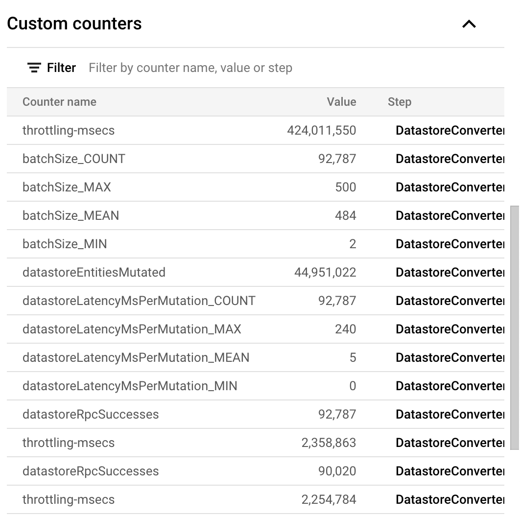
As example a job to delete 44,951,022 entities with default autoscaling took 1 hr 39 min or about 7,567 entities / sec. Here are the complete stats:
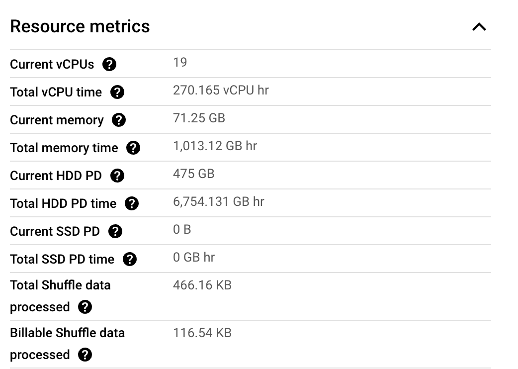
One of the problems with Dataflow is that Google does not provide the cost of a job. However, you can estimate it yourself using the information on their site. In this particular case, this job consumed following resource metrics:
These metrics are staggering btw! How much do you think the job would have cost? Think about it. We can calculate it as:
This post summarizes results of performance benchmarking some databases. For our test, we use a dataset similar to the Star Schema Benchmark and evaluate the performance on following queries:
what is the time to insert a line order item?
what is the time to fetch all the line orders for a customer?
we created a dataset with 44 M line orders. All databases (except Datastore which is serverless) use 8 vCPU and 32 GB RAM. For MySQL this resulted in a table with data_length = 7,269,679,104 bytes. below are the results:
Task
MySQL
AlloyDB
MongoDB
RocksDB
Google Datastore
BigTable
Load all 44 M rows
30 min 35.524 sec (24,491 rows/s)
17 min 53.975 s (41,857 rows/s)
10 min 5s
8 min 12 s
140 min
17 min 39 s
Time to insert new row
5 ms
5 ms
1 ms
< 1 ms
115 ms
1000 ms
Time to fetch all line orders corresponding to a customer
1-2 ms
2 ms
9 ms
8 ms
134 ms
700 ms
How data was loaded
LOAD DATA LOCAL INFILE
\copy FROM ...
Node.js
How tests were done
MySQL CLI
AlloyDB CLI (Postgres)
MongoDB CLI
RocksJava
Node.js
Java
Overall, MySQL, AlloyDB, RocksDB and MongoDB perform close to each other and the numbers are inconclusive so as to suggest one over the other. The results confirm the belief that B-Tree based databases are optimized for minimizing the seek time to read whereas Log Structured Merge Tree (SS Table) databases are optimized for write throughput. The times for Datastore and BigTable are significantly higher presumably because they include the overhead of a network call. However, the network call happens in case of MySQL also when using the CLI (MySQL client calls remote MySQL server) and when we benchmarked MySQL with a Node.js application using the mysql2 driver, response times were practically the same as when using the CLI.
For MySQL there is almost a 6x improvement (in time) if the records are inserted in PK order, not to mention reduced data size (data_length). See this for example.
The results are not intended to suggest any database over another. There are many other factors to consider when making a decision.
AlloyDB is a new HTAP database that Google claims to give 4x better OLTP performance than Postgres. Here, we describe a performance test to compare its performance to Postgres as I wanted to see it for myself. TL;DR: For the tests we did, we find the performance is the same with little to no difference at all. This is not to challenge Google’s claim as the results vary depending on how the databases are configured, what data is stored and what queries are run etc.
The Setup
For our Postgres server we use a VM with 8 vCPU, 32 GB RAM and 250 GB SSD. This costs $447 / month. Refer this.
For our AlloyDB server we use a VM with 4 vCPU, 32 GB RAM and 250 GB SSD. This costs 48.24*4+8.18*32+0.3*250 = $530 / month. Refer this. Although a VM with 2 vCPU would be closer in cost to $447, the GCloud console did not provide that configuration as an option.
shared_buffers is an important setting and is found to be set to 10704 MB for Postgres and 25690 MB for AlloyDB by GCloud – we did not customize the settings.
We downloaded and installed sysbench 1.0.20 on Debian. Log file. sysbench test scripts are located under /usr/share/sysbench.
Preparing Test Table
A test table with 1B rows was created in both Postgres and AlloyDB using following command as example:
This is what we found (tx/s = transactions per second):
Test
Postgres (tx/s)
AlloyDB (tx/s)
oltp_read_write
6.63
9.16
oltp_delete
2540.65
2532
oltp_insert
2398
2417
oltp_point_select
2547
2567
oltp_read_only
152
160
oltp_update_index
2551
2564
oltp_update_non_index
2549
2566
oltp_write_only
23
19
select_random_points
2543
2561
select_random_ranges
2513
2541
Conclusion
The results are practically the same with little to no difference. What about MySQL? We did perform the same analysis on MySQL 8.0 (using similar VM as Postgres). Here are the results:
Task
create table with 1B rows
672m18.342s
data_length
207,806,791,680
Running the sysbench tests however gave this error: Commands out of sync; you can't run this command now and prevented further testing. This is a bug in sysbench fixed in this commit but not released at time of this writing. I am actually surprised how people use sysbench to test MySQL when its broken out of the box.
AlloyDB can be very fast (comparable to any other state-of-the-art real-time analytics db) but only if the entire columns on which a query depends can be fit into the memory of its columnar engine.
This constraint does not scale. we can’t keep increasing RAM to accommodate ever-increasing datasets.
Background
Historically two distinct database access patterns emerged – OLTP and OLAP – and databases were developed to cater to either OLTP or OLAP. OLTP databases would capture data from transactional systems (e.g., sales orders) and the data would be copied to an OLAP database or warehouse for analysis through a process known as ETL. Entire companies made (and continue to make) their livelihood developing ETL software which is just a fancy term to copy data from one db to another (there is also transformation of the data but its optional and we ignore it for the moment). However, as data volumes grow to ever-increasing sizes, copying the data becomes expensive both in terms of cost and time. In some cases by the time the data hits OLAP database, it is already stale (i.e., OLAP database is always lagging behind the real-time OLTP systems). Also consider the emergence of user-facing analytical applications. E.g., Uber has a treasure trove of ride data. An application can be built that would allow a user to select a starting and ending point on a map, a radius around start and end points (1 km as example), and a time-period (e.g., past 1 month), and it would fetch all the rides that satisfy those constraints and display the average time, std deviation, even the histogram etc. all in real-time, on-demand using the most up-to-date data. It is not possible to pre-compute the results for all possible inputs a user may enter: the range of inputs is practically infinite.
How do we make this possible? To address above problems and new use-cases, a new breed of databases has now emerged – so-called Hybrid Transactional and Analytical Processing or HTAP databases. These databases aim to unify OLTP and OLAP so that you don’t have to maintain two systems, copy data back and forth, and can run both types of workloads from a single database. There are tons of examples: Snowflake’s Unistore, SingleStore, Amazon Aurora, MySQL HeatWave, TiDB, Citus etc. This brings us to AlloyDB which is Google’s foray into this area.
The way all these databases work is by maintaining both a OLTP (row-based) and OLAP (columnar engine) store underneath and automatically routing a query to either OLTP or OLAP depending on which will be faster. The database also takes care of syncing the data between the two stores.
Performance Benchmarking of AlloyDB
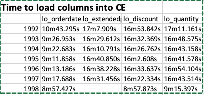
The performance of AlloyDB was measured on the Star Schema Benchmark with 2B line order items (250 GB dataset). A cluster with 64 GB RAM (8 vCPUs) was provisioned and 32 GB of RAM was dedicated to the columnar engine. We were only able to load a few of the columns into the columnar engine because of the size limitations. It actually took 6.5 hours! to load the lineorder table from a CSV file (compare to 30 min for ClickHouse). Creating the denormalized table (lineorder_flat) took another 10.5 hours!! and loading the lo_quantity, lo_extendedprice, lo_discount, lo_orderdate columns into the CE (columnar engine) took us following times:
So it was not an easy process by all means. We partitioned the table by year using following commands as example:
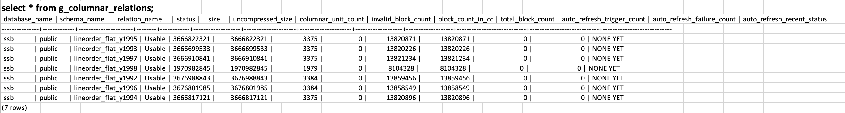
Once the columns are loaded, we can observe the space taken as follows (click on the image to enlarge):
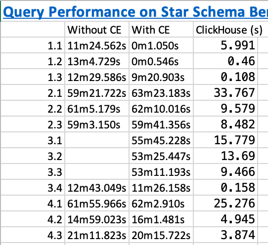
And below are the execution times on the SSB queries before we added the columns and after we added the columns. The execution time of ClickHouse is shown for comparison:
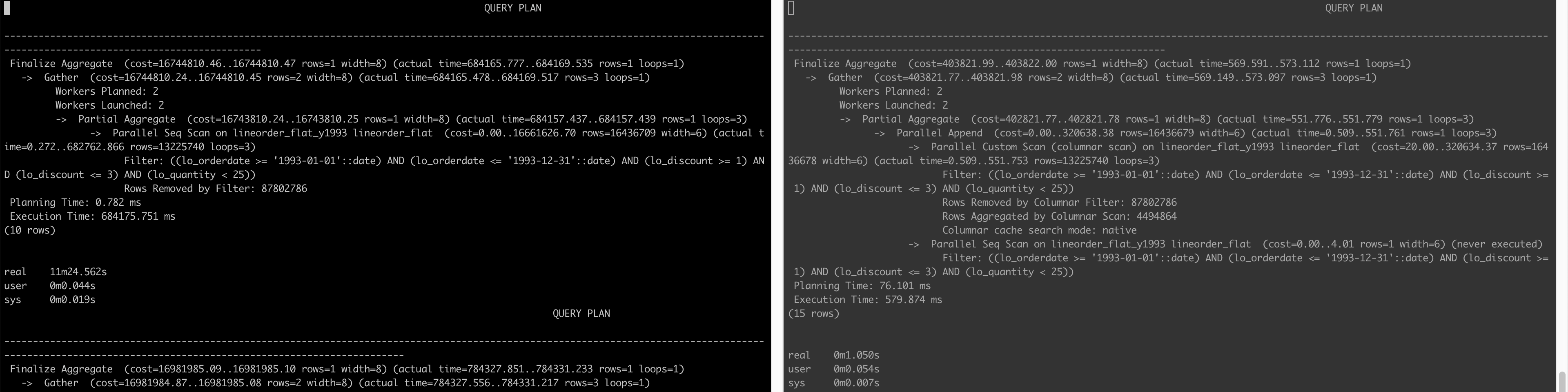
Below is the query plan that compares how a query is executed when not using the CE (left) and when AlloyDB is able to use the CE (right) (click on the image to enlarge)
Conclusion
The lesson learned here is that yes AlloyDB can be very fast (6000x faster!!! for query 1.2 as example when we looked at actual execution time 784337 ms vs. 127 ms) but only if the entire columns on which a query depends can be fit into its RAM (doesn’t matter if the column is in WHERE clause or SELECT clause or any other clause for that matter) – this is not a realistic constraint.
Other Notes
PostgreSQL provides Extract(year from date) method to get the year of a date column. However, using Extract(year from date) as below e.g.:
SELECT sum(LO_EXTENDEDPRICE * LO_DISCOUNT) AS revenue
FROM lineorder_flat
WHERE extract(year from LO_ORDERDATE) = 1993 AND LO_DISCOUNT BETWEEN 1 AND 3 AND LO_QUANTITY < 25;
PostgreSQL (and thus AlloyDB) was still searching all the partitions. We have to rewrite the query as:
SELECT sum(LO_EXTENDEDPRICE * LO_DISCOUNT) AS revenue
FROM lineorder_flat
WHERE LO_ORDERDATE >= '1993-01-01' and lo_orderdate <= '1993-12-31' AND LO_DISCOUNT BETWEEN 1 AND 3 AND LO_QUANTITY < 25;
for it to only search within the 1993 partition.
Similarly, query 1.3 takes long even though all the columns it depends on are in the CE. This is because of the presence of extract(week from LO_ORDERDATE) in the query:
SELECT sum(LO_EXTENDEDPRICE * LO_DISCOUNT) AS revenue
FROM lineorder_flat
WHERE extract(week from LO_ORDERDATE) = 6 AND LO_ORDERDATE >= '1994-01-01' and lo_orderdate <= '1994-12-31'
  AND LO_DISCOUNT BETWEEN 5 AND 7 AND LO_QUANTITY BETWEEN 26 AND 35;
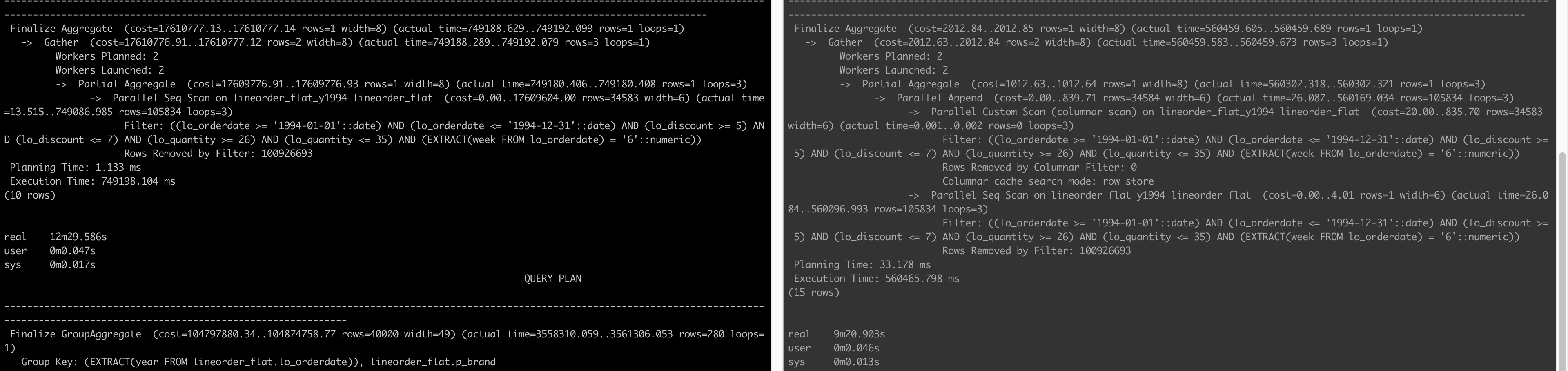
Below are the query plans before adding columns to CE and after:
We see on the right that although it does a Parallel Custom Scan (columnar scan), the Columnar cache search mode is row store as opposed to native in queries 1.1 and 1.2. In the end, the column store is not able to make the query faster.
The trick to make the query run fast is to rewrite it as:
SELECT sum(LO_EXTENDEDPRICE * LO_DISCOUNT) AS revenue
FROM lineorder_flat
WHERE LO_ORDERDATE >= '1994-02-07' and lo_orderdate <= '1994-02-13'
  AND LO_DISCOUNT BETWEEN 5 AND 7 AND LO_QUANTITY BETWEEN 26 AND 35;
This query executes in just 108 ms with following query plan:
                                                                                                   QUERY PLAN
-----------------------------------------------------------------------------------------------------------------------------------------------------------------------------------------------------------------
 Finalize Aggregate  (cost=4233.50..4233.51 rows=1 width=8) (actual time=98.859..102.062 rows=1 loops=1)
   ->  Gather  (cost=4233.28..4233.49 rows=2 width=8) (actual time=98.559..102.048 rows=3 loops=1)
         Workers Planned: 2
         Workers Launched: 2
         ->  Partial Aggregate  (cost=3233.28..3233.29 rows=1 width=8) (actual time=90.280..90.282 rows=1 loops=3)
               ->  Parallel Append  (cost=0.00..2602.86 rows=126084 width=6) (actual time=0.895..90.266 rows=1 loops=3)
                     ->  Parallel Custom Scan (columnar scan) on lineorder_flat_y1994 lineorder_flat  (cost=20.00..2598.85 rows=126083 width=6) (actual time=0.894..90.258 rows=105834 loops=3)
                           Filter: ((lo_orderdate >= '1994-02-07'::date) AND (lo_orderdate <= '1994-02-13'::date) AND (lo_discount >= 5) AND (lo_discount <= 7) AND (lo_quantity >= 26) AND (lo_quantity <= 35))
                           Rows Removed by Columnar Filter: 100926693
                           Rows Aggregated by Columnar Scan: 37446
                           Columnar cache search mode: native
                     ->  Parallel Seq Scan on lineorder_flat_y1994 lineorder_flat  (cost=0.00..4.01 rows=1 width=6) (never executed)
                           Filter: ((lo_orderdate >= '1994-02-07'::date) AND (lo_orderdate <= '1994-02-13'::date) AND (lo_discount >= 5) AND (lo_discount <= 7) AND (lo_quantity >= 26) AND (lo_quantity <= 35))
 Planning Time: 25.348 ms
 Execution Time: 108.731 ms
(15 rows)
And finally…
The application described in the background section was actually developed at Uber and is called Uber Movement. When it was developed in 2016, HTAP databases had not appeared and so what we did is to discretize a city into zones with fixed boundaries. User could not select any arbitrary start and end points on the map, they could select start and end zones. This allowed us to reduce the range of possibly infinite inputs to a more finite number and then we precomputed aggregates to serve the analytics to the user from the web interface. Computing the aggregates in real-time,on-demand was infeasible with the tools we had at that time. You can read more about the whole process in this whitepaper.
Always create your own primary key. [ref]. The PK controls how your data is physically laid out.
Always try to insert records in PK order [ref]. Usually this means use AUTO_INCREMENT for the PK. Using UUID is a very poor choice. A commonly encountered situation is when you are ingesting data from elsewhere and the data already uses a UUID to uniquely identify records. In this case you are stuck between a rock and a hard place. – Option 1: You use AUTO_INCREMENT for PK. Your writes will be fast but you lose any data-integrity checks and you won’t be able to lookup by UUID (reads are slow). – Option 2: You use the UUID field for PK. You are guaranteed data-integrity (no duplicates) but your writes will suffer and index will bloat up significantly. – Option 3: You use AUTO_INCREMENT for PK and CREATE UNIQUE INDEX on the UUID column. I suspect this will give same performance (or worse) than Option 2. – Option 4 (not always possible): Use Option 3 but disable the index when doing inserts [ref]. Only works when you are able to do inserts in bulk. Not possible if you need to do inserts continuously as is the case in lot of applications.
For high-performance applications, don’t use FKs. Rely on your application to maintain data-integrity.
For high-performance, avoid SELECT ... FOR UPDATE and instead rely on application-level optimistic concurrency control using a version column.
Single most important setting to get right is the innodb_buffer_pool_size. Set it large enough so your indexes can fit in memory. But it should be less than 75% of RAM. Give some space to the OS, connections etc. Do some research on SO etc.