
TL;DR:
- AlloyDB can be very fast (comparable to any other state-of-the-art real-time analytics db) but only if the entire columns on which a query depends can be fit into the memory of its columnar engine.
- This constraint does not scale. we can’t keep increasing RAM to accommodate ever-increasing datasets.
Background
Historically two distinct database access patterns emerged – OLTP and OLAP – and databases were developed to cater to either OLTP or OLAP. OLTP databases would capture data from transactional systems (e.g., sales orders) and the data would be copied to an OLAP database or warehouse for analysis through a process known as ETL. Entire companies made (and continue to make) their livelihood developing ETL software which is just a fancy term to copy data from one db to another (there is also transformation of the data but its optional and we ignore it for the moment). However, as data volumes grow to ever-increasing sizes, copying the data becomes expensive both in terms of cost and time. In some cases by the time the data hits OLAP database, it is already stale (i.e., OLAP database is always lagging behind the real-time OLTP systems). Also consider the emergence of user-facing analytical applications. E.g., Uber has a treasure trove of ride data. An application can be built that would allow a user to select a starting and ending point on a map, a radius around start and end points (1 km as example), and a time-period (e.g., past 1 month), and it would fetch all the rides that satisfy those constraints and display the average time, std deviation, even the histogram etc. all in real-time, on-demand using the most up-to-date data. It is not possible to pre-compute the results for all possible inputs a user may enter: the range of inputs is practically infinite.
How do we make this possible? To address above problems and new use-cases, a new breed of databases has now emerged – so-called Hybrid Transactional and Analytical Processing or HTAP databases. These databases aim to unify OLTP and OLAP so that you don’t have to maintain two systems, copy data back and forth, and can run both types of workloads from a single database. There are tons of examples: Snowflake’s Unistore, SingleStore, Amazon Aurora, MySQL HeatWave, TiDB, Citus etc. This brings us to AlloyDB which is Google’s foray into this area.
The way all these databases work is by maintaining both a OLTP (row-based) and OLAP (columnar engine) store underneath and automatically routing a query to either OLTP or OLAP depending on which will be faster. The database also takes care of syncing the data between the two stores.
Performance Benchmarking of AlloyDB
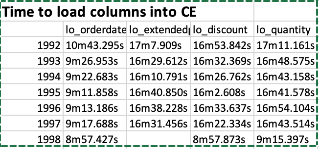
The performance of AlloyDB was measured on the Star Schema Benchmark with 2B line order items (250 GB dataset). A cluster with 64 GB RAM (8 vCPUs) was provisioned and 32 GB of RAM was dedicated to the columnar engine. We were only able to load a few of the columns into the columnar engine because of the size limitations. It actually took 6.5 hours! to load the lineorder table from a CSV file (compare to 30 min for ClickHouse). Creating the denormalized table (lineorder_flat) took another 10.5 hours!! and loading the lo_quantity, lo_extendedprice, lo_discount, lo_orderdate columns into the CE (columnar engine) took us following times:
So it was not an easy process by all means. We partitioned the table by year using following commands as example:
CREATE TABLE lineorder
(
    row_id serial,
    LO_ORDERKEY             integer,
    LO_LINENUMBER           integer,
    LO_CUSTKEY              integer,
    LO_PARTKEY              integer,
    LO_SUPPKEY              integer,
    LO_ORDERDATE            Date,
    LO_ORDERPRIORITY        varchar(99),
    LO_SHIPPRIORITY         smallint,
    LO_QUANTITY             smallint,
    LO_EXTENDEDPRICE        integer,
    LO_ORDTOTALPRICE        integer,
    LO_DISCOUNT             smallint,
    LO_REVENUE              integer,
    LO_SUPPLYCOST           integer,
    LO_TAX                  smallint,
    LO_COMMITDATE           Date,
    LO_SHIPMODE             varchar(99),
    junk varchar(4),
    primary key (lo_orderdate, serial)
) PARTITION BY RANGE (lo_orderdate);

CREATE TABLE lineorder_y1991 PARTITION OF lineorder FOR VALUES FROM ('1991-01-01') TO ('1992-01-01');
The command to load a column is (illustrated with an example):
SELECT google_columnar_engine_add('lineorder_flat_y1994', 'lo_orderdate');
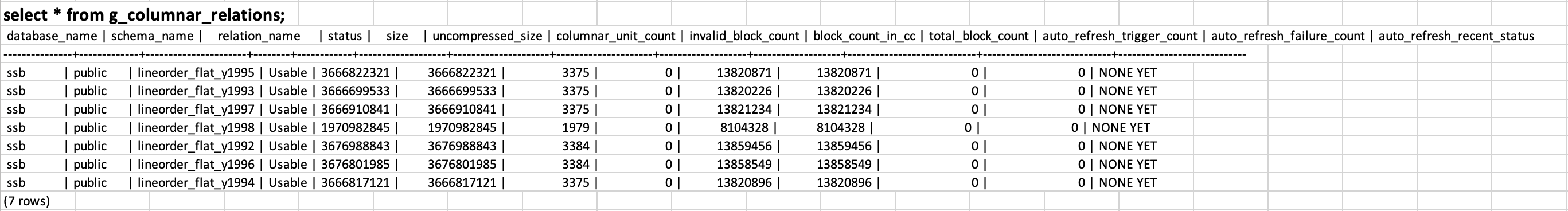
Once the columns are loaded, we can observe the space taken as follows (click on the image to enlarge):
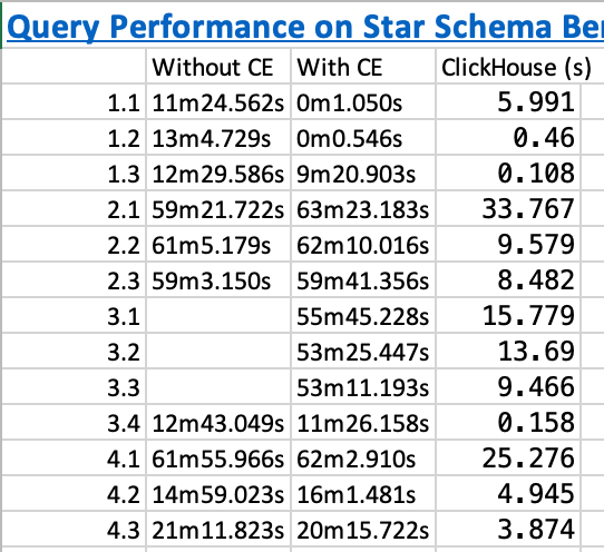
And below are the execution times on the SSB queries before we added the columns and after we added the columns. The execution time of ClickHouse is shown for comparison:
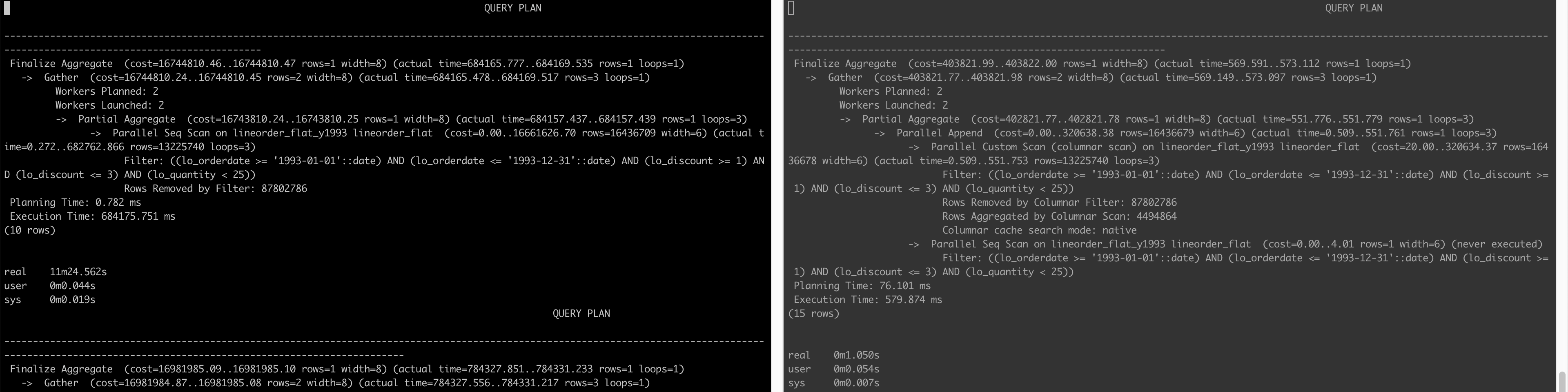
Below is the query plan that compares how a query is executed when not using the CE (left) and when AlloyDB is able to use the CE (right) (click on the image to enlarge)
Conclusion
The lesson learned here is that yes AlloyDB can be very fast (6000x faster!!! for query 1.2 as example when we looked at actual execution time 784337 ms vs. 127 ms) but only if the entire columns on which a query depends can be fit into its RAM (doesn’t matter if the column is in WHERE clause or SELECT clause or any other clause for that matter) – this is not a realistic constraint.
Other Notes
PostgreSQL provides Extract(year from date) method to get the year of a date column. However, using Extract(year from date) as below e.g.:
SELECT sum(LO_EXTENDEDPRICE * LO_DISCOUNT) AS revenue
FROM lineorder_flat
WHERE extract(year from LO_ORDERDATE) = 1993 AND LO_DISCOUNT BETWEEN 1 AND 3 AND LO_QUANTITY < 25;
PostgreSQL (and thus AlloyDB) was still searching all the partitions. We have to rewrite the query as:
SELECT sum(LO_EXTENDEDPRICE * LO_DISCOUNT) AS revenue
FROM lineorder_flat
WHERE LO_ORDERDATE >= '1993-01-01' and lo_orderdate <= '1993-12-31' AND LO_DISCOUNT BETWEEN 1 AND 3 AND LO_QUANTITY < 25;
for it to only search within the 1993 partition.
Similarly, query 1.3 takes long even though all the columns it depends on are in the CE. This is because of the presence of extract(week from LO_ORDERDATE) in the query:
SELECT sum(LO_EXTENDEDPRICE * LO_DISCOUNT) AS revenue
FROM lineorder_flat
WHERE extract(week from LO_ORDERDATE) = 6 AND LO_ORDERDATE >= '1994-01-01' and lo_orderdate <= '1994-12-31'
  AND LO_DISCOUNT BETWEEN 5 AND 7 AND LO_QUANTITY BETWEEN 26 AND 35;
Below are the query plans before adding columns to CE and after:
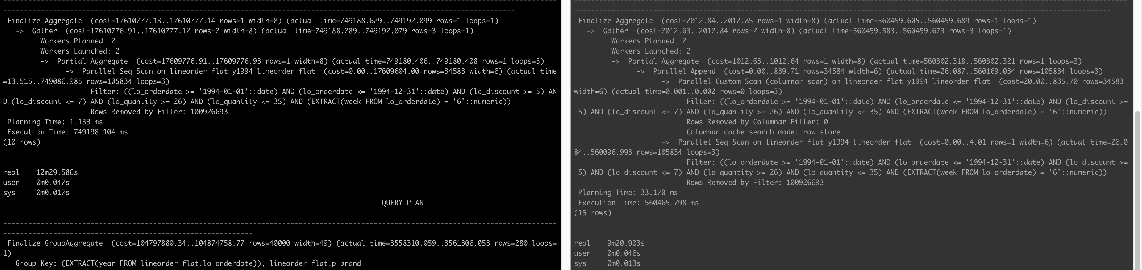
We see on the right that although it does a Parallel Custom Scan (columnar scan), the Columnar cache search mode is row store as opposed to native in queries 1.1 and 1.2. In the end, the column store is not able to make the query faster.
The trick to make the query run fast is to rewrite it as:
SELECT sum(LO_EXTENDEDPRICE * LO_DISCOUNT) AS revenue
FROM lineorder_flat
WHERE LO_ORDERDATE >= '1994-02-07' and lo_orderdate <= '1994-02-13'
  AND LO_DISCOUNT BETWEEN 5 AND 7 AND LO_QUANTITY BETWEEN 26 AND 35;
This query executes in just 108 ms with following query plan:
                                                                                                   QUERY PLAN
-----------------------------------------------------------------------------------------------------------------------------------------------------------------------------------------------------------------
 Finalize Aggregate  (cost=4233.50..4233.51 rows=1 width=8) (actual time=98.859..102.062 rows=1 loops=1)
   ->  Gather  (cost=4233.28..4233.49 rows=2 width=8) (actual time=98.559..102.048 rows=3 loops=1)
         Workers Planned: 2
         Workers Launched: 2
         ->  Partial Aggregate  (cost=3233.28..3233.29 rows=1 width=8) (actual time=90.280..90.282 rows=1 loops=3)
               ->  Parallel Append  (cost=0.00..2602.86 rows=126084 width=6) (actual time=0.895..90.266 rows=1 loops=3)
                     ->  Parallel Custom Scan (columnar scan) on lineorder_flat_y1994 lineorder_flat  (cost=20.00..2598.85 rows=126083 width=6) (actual time=0.894..90.258 rows=105834 loops=3)
                           Filter: ((lo_orderdate >= '1994-02-07'::date) AND (lo_orderdate <= '1994-02-13'::date) AND (lo_discount >= 5) AND (lo_discount <= 7) AND (lo_quantity >= 26) AND (lo_quantity <= 35))
                           Rows Removed by Columnar Filter: 100926693
                           Rows Aggregated by Columnar Scan: 37446
                           Columnar cache search mode: native
                     ->  Parallel Seq Scan on lineorder_flat_y1994 lineorder_flat  (cost=0.00..4.01 rows=1 width=6) (never executed)
                           Filter: ((lo_orderdate >= '1994-02-07'::date) AND (lo_orderdate <= '1994-02-13'::date) AND (lo_discount >= 5) AND (lo_discount <= 7) AND (lo_quantity >= 26) AND (lo_quantity <= 35))
 Planning Time: 25.348 ms
 Execution Time: 108.731 ms
(15 rows)
And finally…
The application described in the background section was actually developed at Uber and is called Uber Movement. When it was developed in 2016, HTAP databases had not appeared and so what we did is to discretize a city into zones with fixed boundaries. User could not select any arbitrary start and end points on the map, they could select start and end zones. This allowed us to reduce the range of possibly infinite inputs to a more finite number and then we precomputed aggregates to serve the analytics to the user from the web interface. Computing the aggregates in real-time, on-demand was infeasible with the tools we had at that time. You can read more about the whole process in this whitepaper.
